Over the last few posts, I've been testing how Strava's Privacy Zones hold up in practice. So far, the results haven't been encouraging: with only a few activities, it's possible to reverse-engineer the start location and while increasing the privacy zone size does help, it doesn't solve the problem.
I've also looked at different environments. In cities, where start points are fairly well distributed, simple geometric methods work reasonably well. But in rural areas - villages, cul-de-sacs or long driveways - the same methods struggle. With so little spread in the data, there isn't much for them to work with.
So far, I've only used basic geometric methods, and they have obvious limits. The natural question is: what happens if I try something different - something a bit more sophisticated that uses the road network to address those weaknesses?
Let's try exactly that.
Weaknesses of Current Methods
Before building a more sophisticated method, it's worth looking at the weaknesses of the current geometric approaches and where they fall short:
- Dependence on point distribution: If start points aren't well spread, the methods struggle or fail entirely. This is especially obvious in rural areas, where a handful of start locations doesn't provide enough data.
- Ignoring the road network: Current methods treat space geometrically but don't consider how people actually move along roads or paths. In rural areas, where there are few route options, this is essential.
- Neglecting Strava metadata: Aside from the Adaptive Donuts Method, no method uses metadata like the hidden distance in the privacy zone. Incorporating this could drastically improve predictions.
- Ignoring initial activity direction: People usually head straight away from home for the first few hundred meters. Factoring in this direction could help guide predictions, especially in sparse locations.
The first weakness is obvious in rural tests: without a good spread of start points, geometric methods struggle. The second weakness can be addressed by factoring in the road network, which is particularly powerful where options are limited. The third weakness - using the hidden distance - works alongside the road network to pinpoint where the true start is likely to be. And the fourth can be combined with the others to tackle special cases like cul-de-sacs or single driveways: if we know how far the hidden section is, we can move in the opposite direction along the road to find the true start.
A Different Approach - The “Homing” Method
The idea behind the “Homing” method is simple in concept: for each start location at the edge of the privacy zone, I plot lots of possible routes into the privacy zone along the road network. I then compare the distance of each route to the hidden distance recorded in the Strava metadata. The point in the privacy zone with the smallest total error across all start locations should, in theory, be closest to the true start location.
Here's how it works step by step:
- Identify an approximate area for the true start - a "hot" zone that contains it.
- Grab the road network for that area and overlay a grid.
- For each grid point, plot routes to each start location along the road network.
- Compare the distance of each plotted route to the hidden distance from Strava.
- Pick the grid point with the lowest total error across all start locations - that's the best guess.
- Zoom in: shrink the grid around this best guess and repeat until it converges on the true start.
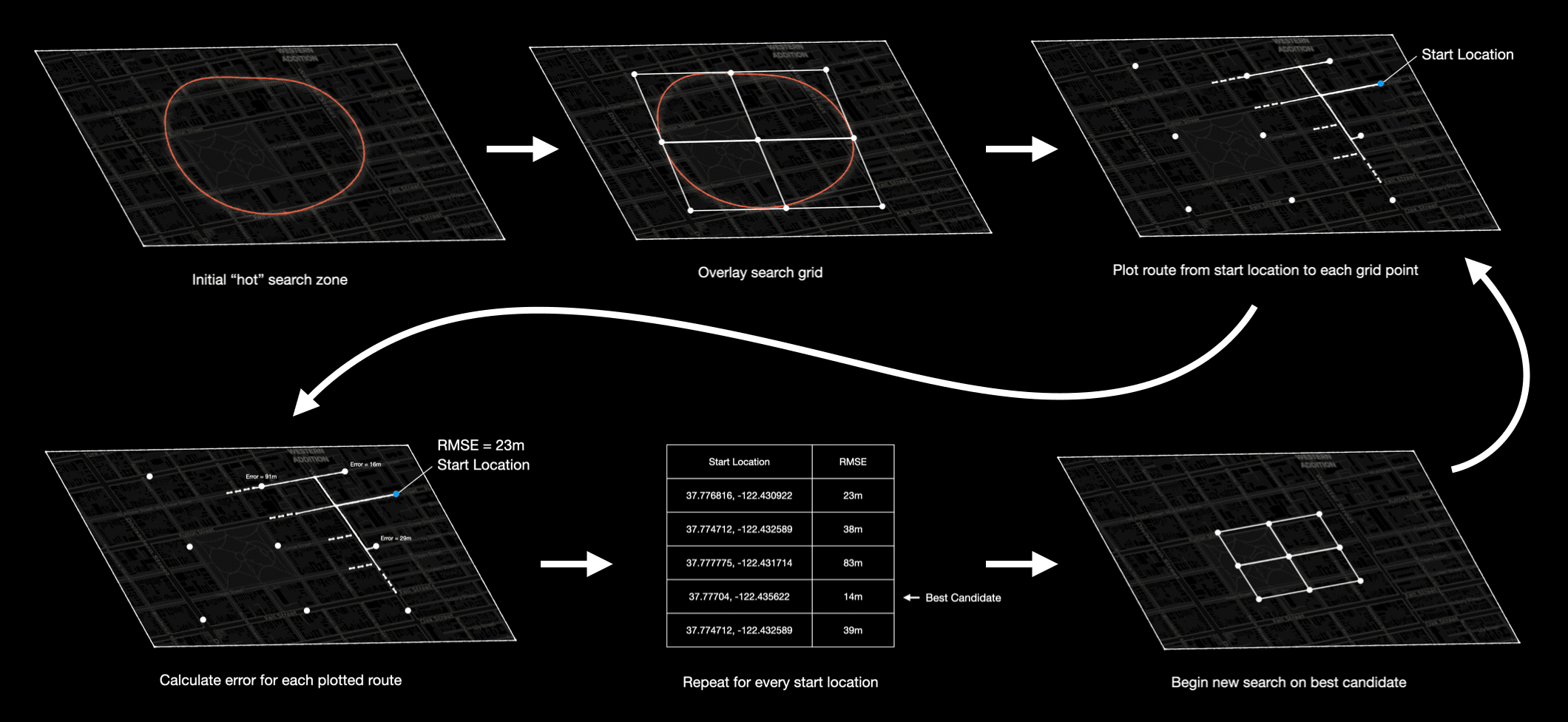
The "Homing" Method
Sounds simple enough, putting it into practice is slightly trickier.
How It Works (And What Went Wrong Along the Way)
Building the Method
The first challenge is finding an approximate area for the true start location. Luckily, I already have a method for this: the "hot" zones from the Adaptive Donuts Method heatmaps consistently contained the true start in all my experiments, so I can reuse them here. Technically, you could search the entire area containing all start points, but using the "hot" zone instantly reduces the search space, so seems helpful.
Getting the road network is straightforward using OSMnx - I already did this back in post I for route generation. Creating a grid over this area is also simple. In this case, I took the "hot" zone from the Adaptive Donuts Method (calculated using clustering), drew a bounding box around it and split it into a grid of points. I use odd dimensions, like 3x3, 5x5 or 7x7, to ensure there's always a centre point. For future refinements, I set the best guess as the grid's centre, so the search focuses around it. There are other ways to do this, of course, but this approach is intuitive and easy to implement.
Deciding when to conclude the search - and how to refine the grid - is always a key question. I explored different options and settled on a maximum of 6 iterations, using a 3x3 grid with spacing halving each time, based on the "hot" zone extremes. I also included a threshold for early termination, but with only 6 iterations and the search being fast, I set it so low it's rarely triggered. More detail is in the grid search parameter experimentation section after the results.
Plotting routes from each grid point to the start locations is straightforward with OSMnx, it uses Dijkstra's algorithm by default to find the shortest path along the road network. This assumes the plotted route from the edge of the privacy zone to the true start is the shortest path - a reasonable assumption since most people head straight away from home at the start of an activity.
The final step is looping through all grid points (snapped to the nearest point in the road network), plotting routes to each start location, calculating errors and selecting the grid point with the lowest error. I use Root Mean Square Error (RMSE) as the metric:
Calculating the hidden distance uses the Strava metadata on the activity. The activity distance includes the portion inside the privacy zone (since people don't want to lose this from their activity) and the downloaded route excludes it. Subtracting the plotted route distance from the total activity distance gives the distance covered in the privacy zone. I divide this by two, since it accounts for both the start and end of the activity, giving an approximate hidden distance for the start portion.
Hidden Distance Calculation
The Early Snags
I tried this approach, but ran into a few issues.
First, OSMnx's route plotting algorithm isn't great. It often takes the long way around, which makes the plotted route distances inaccurate - a problem, since this method relies on precise distances. There are a few reasons for this: it's a simple algorithm, the road network data isn't always detailed enough, and in some areas (especially rural ones) the graph coverage is limited - I even saw roads missing entirely. On top of that, the accuracy of edge lengths can vary, which further skews results.
The solution was to run a local OSRM server as the routing engine. This is lightweight, much more accurate than OSMnx, and faster.
I downloaded the OSM data for each start location area, loaded the appropriate OSRM profile (car, but foot or bike could work too),
and made route calculations via HTTP requests GET /route/v1/{profile}/{lon1},{lat1};{lon2},{lat2}. This gave the precision I
needed for the method to function properly.
During some early city runs, I got perfect predictions - 0.0m error - which immediately seemed suspicious. The issue was with snapping: both the true start location and the grid points were snapping to the same point on the map, giving an unfair advantage. I could have regenerated the routes, but a better fix was to improve snapping. By default, grid points snap to the nearest node or junction, but I rewrote the algorithm to snap to the nearest edge instead. Points are then projected onto the edge, so they can sit mid-edge rather than only at nodes.
Finally, I experimented with different error metrics. Some produced wildly different results, so I stuck with RMSE. It proved the most consistent and reliable across the board.
Results
City
Here are the results for the homing method in the city location.
I expected this method to perform well in the city, but not dramatically better than the geometric methods. With a good distribution of start points, the geometric methods already do reasonably well. I also assumed the abundance of possible routes might make the homing method prone to small errors.
Surprisingly, it did better than I expected. The homing method predicted the start location most accurately of all the methods - to within 18.5m, 10m closer than the best geometric approach.
I also tested larger privacy zones, up to 800m. For a 400m privacy zone, the predicted start was 57.6m from the true location; for 800m, it was 246.3m away. The 800m result is noticeably worse than the geometric methods (Adaptive Donuts Method: 188.6m, being the current worst), while the 400m prediction falls roughly in the same range as the geometric approaches.
This isn't too surprising. In a city, there are countless route options, so small deviations and errors compound quickly. I'm sure further refinements could improve the results, but it's a good start.
City Grid
The city grid location performs well, it's a good prediction and better than some of the others, but it's no home run. This is what I kind of expected from the city location, a reasonable prediction, but nothing standout. In cities there are just lots of possible combinations and routes. On reflection this city grid contains more possible routes than the original city location, which is less regular, and might be the reason for the increased challenge.
The homing method does well in the city grid location - a solid prediction, better than some of the other methods, but it's no home run. This is what I expected: in cities, there are just so many possible route combinations that this method can only go so far.
Looking closer, this city grid is actually more challenging than the original city location. Its regular layout creates more route options, which likely explains why the prediction isn't a standout. Still, it's a respectable result and confirms the method is at least competitive in dense urban environments.
Rural
Now we get to the part the method was really built for: rural locations, where route options are limited. And it does not disappoint. The homing method predicts the start to within an astonishing 5.6m - almost 40m better than the next best method. In other words, it has basically found the front door. Frankly, this is terrifying.
Even with fewer activities, it still performs remarkably well. With just 10 activities, the prediction is within 28m, and it gradually tightens to 5.6m with 40 activities. Unlike geometric methods, which can be thrown off by outliers, the homing method's performance scales predictably: 21.1m for 20 activities, 10.2m for 30.
Put simply: with just 10 activities, you can predict someone's home in a rural area to within a stone's throw. With more activities, you get even closer - down to a car-length from the true start. Let that sink in: Strava privacy zones, even when applied, offer almost no protection here.
A larger privacy zone doesn't help much either. With a 400m radius, the prediction is 12.1m from the true start; at 800m, it's 32.5m. For comparison, the next best geometric method (Adaptive Donuts Method) only manages 182.6m.
Cul-de-sac
The homing method doesn't directly work for cul-de-sacs, since the predicted start location could fall on either side of the cluster of start points. The solution? Simply head in the opposite direction to the activity from each start point, into the "cul-de-sac", using the hidden distance from the Strava metadata (in this case, 311m on average). With two possible routes through the "cul-de-sac" it gives two predictions instead of one.
This approach is very effective, landing within 53-84m of the true start location. In this example, the two predictions are close together, but in more complex cul-de-sacs they could differ significantly. Even so, for single-driveway or sparsely populated cul-de-sacs, this is usually enough to pinpoint the home. Often, there are only a few nearby houses, so identifying the correct one visually becomes trivial. In short: unless you max out your privacy zone or live in a dense cul-de-sac, it's easy to reverse-engineer the start location down to ~50m - essentially revealing the home.
When testing larger privacy zones, the results are interesting. For a 400m radius, the average hidden distance is 498m. Applying this in the opposite direction from the start point cluster gives two possible predictions, landing 58.9m and 88.9m from the true start location. That's only a few metres further out than the 200m case, so increasing the radius has very little effect.
With an 800m privacy zone, the average hidden distance jumps to 840m - longer than the road from the start locations to the end (~780m). This happens partly because Strava's processing affects larger privacy zones and partly due to a few outlier activities that stretch the calculated distance. There are a few ways to handle this: you could reduce the distance, take the minimum instead of the average, or simply assume the end location is at the road's end - which in this case is exactly the case.
Either way, the result is still remarkably accurate. Even with an 800m privacy zone, the predicted points fall between 0.0m and 137.9m, with one perfect and the other a reasonable worst-case - still much closer than the privacy zone would suggest.
In these sparse environments, larger privacy zones are largely a fiction - more of a cosmetic disguise than real protection. Even at 800m, they barely change the outcome. Plus since there is no distribution in start points, a single activity is enough to get an accurate prediction; additional activities just fine-tune it.
Summary
The homing method really shines where there are few possible routes - in rural areas, it's ultra-precise. In cities, with many overlapping paths, it's naturally harder. Even on large privacy zones, it nails rural locations to within 32m for an 800m radius - way better than any other method. Honestly, with further tweaking, it could probably do even better.
How I Selected the Grid Search Parameters for the Homing Method
I ran a few experiments to see what grid search parameters worked best for this method - mostly trying to balance accuracy and speed. The main variables I looked at were grid size, grid reduction factor, error metric and the number of top candidates to keep each iteration.
Grid Size: 3x3 vs 7x7
The first thing I looked at was the grid size. The obvious choice seems a finer grid - more points, more precision. But does it actually help?
I ran both 3x3 and 7x7 grids across the locations and privacy zones.
| Location | Privacy Zone | 3x3 Grid (m) | 7x7 Grid (m) | Difference (m) |
|---|---|---|---|---|
| City | 200m | 18.5 | 18.3 | +0.2 |
| City | 400m | 57.6 | 57.0 | +0.6 |
| City Grid | 200m | 41.7 | 41.7 | 0.0 |
| Rural | 200m | 5.6 | 5.7 | -0.1 |
| Rural | 400m | 49.0 | 49.4 | -0.4 |
| Rural | 800m | 89.3 | 89.9 | -0.6 |
The results were very close - in other words, the extra points didn't buy you much accuracy, but they did slow things down significantly. In rural 200m searches, for example, 3x3 took ~20s while 7x7 took ~80s. For such a small gain, it wasn't worth it.
Takeaways: The 3x3 grid is more than sufficient for these environments, and it's far faster. If anything, the 7x7 grid is overkill for little gain.
Grid Reduction Factor: 0.5 vs 0.33
Next up, I explored how aggressively the grid spacing should shrink each iteration. The options I tested were:
- 0.5 - halve the spacing each iteration
- 0.33 - reduce spacing by a third each iteration (e.g., 90m -> 60m -> 40m)
The idea is simple: smaller reductions give more gradual refinements, but may take more iterations to converge. Here's what I found across the main locations.
| Location | Privacy Zone | 0.5 Reduction (m) | 0.33 Reduction (m) | Difference (m) |
|---|---|---|---|---|
| City | 200m | 18.5 | 19.1 | -0.6 |
| City | 400m | 57.6 | 55.3 | +2.3 |
| City Grid | 200m | 41.7 | 41.6 | +0.1 |
| Rural | 200m | 5.6 | 6.7 | -1.1 |
Takeaways: There's very little difference in accuracy between the two reduction factors. Sometimes 0.33 was slightly better, sometimes worse - overall, halving (0.5) is simple, intuitive, and works just as well.
This also makes the method slightly faster, so 0.5 became my default choice.
Error Metrics: RMSE vs MedAE
I also experimented with different error metrics to see if they could improve accuracy. The main contenders were:
- RMSE (Root Mean Square Error) - penalizes larger errors more strongly
- MedAE (Median Absolute Error) - less sensitive to outliers
Here's how they performed across the locations.
| Location | Privacy Zone | RMSE (m) | MedAE (m) | Difference (m) |
|---|---|---|---|---|
| City | 200m | 18.5 | 33.8 | -15.3 |
| City | 400m | 57.6 | 16.6 | +41.0 |
| City | 800m | 203.2 | 203.2 | 0.0 |
| City Grid | 200m | 41.7 | 39.7 | +2.0 |
| Rural | 200m | 5.6 | 40.7 | -35.1 |
Takeaways:
- Some predictions are much better with MedAE, others much worse, and some are about the same. The effect is highly dependent on the distribution of errors and outliers.
- RMSE is more consistent across locations and scenarios, which is why it was chosen as the default metric.
- Overall, changing the metric did not provide a systematic improvement in accuracy; it's more a matter of how errors happen to be distributed in each case.
Top-N Candidates: N = 1 vs N = 5
I also experimented with keeping multiple candidate grid points at each iteration instead of just the single best one. The idea was to reduce the risk of getting trapped in a local minimum, especially in more complex environments.
I set N = 5, meaning the top 5 candidates (provided they were sufficiently far apart) would progress to the next iteration as the center points for new grids. For comparison, I also tested the standard N = 1 approach.
Here's how it affected accuracy in the rural location.
| Privacy Zone Radius | N = 1 (m) | N = 5 (m) | Difference (m) |
|---|---|---|---|
| 200m | 5.6 | 5.8 | -0.2 |
| 400m | 12.1 | 12.1 | 0.0 |
| 800m | 32.5 | 32.8 | -0.3 |
Takeaways:
- In these experiments, keeping multiple candidates had very little impact on the final prediction - differences were marginal.
- The extra computation is noticeable (more grid points to evaluate), but in these relatively simple environments it didn't improve accuracy.
- This confirms that in sparse rural areas, where options are limited, a single best candidate per iteration is sufficient.
Speed and Performance
People are always curious about speed, so here are a few stats.
As previously mentioned, a 3x3 grid took ~20s while a 7x7 grid took ~80s, in a 200m privacy zone in the rural location.
Smaller privacy zones are slightly faster, since the route calculations are shorter, but the difference isn't huge - roughly 1.2x to 1.5x faster in my tests.
Rural locations are ~2x faster than city locations (~15s vs ~30s). This makes sense: rural networks have fewer roads and fewer possible routes, so there's less to compute.
It's worth noting that while these runtimes are short for the areas I tested, larger regions or more complex road networks could increase computation time. Even so, for most practical cases, this approach remains entirely tractable.
Overall, this lightweight exploration of grid search parameters for the homing method confirmed that my choices - 3x3 grids, 0.5 reduction factor, RMSE error metric, N=1 - strike a reasonable balance between speed and accuracy.
More Rural Tests - Just to Be Sure
What the Extra Tests Show
I didn't want to leave it at a single rural location and claim the method is near perfect in sparse road networks. One location simply isn't enough to make a strong case. So I created three more rural sites, each with 40 activities and a 200m privacy zone, to see whether the homing method really holds up.
The results were reassuringly consistent.
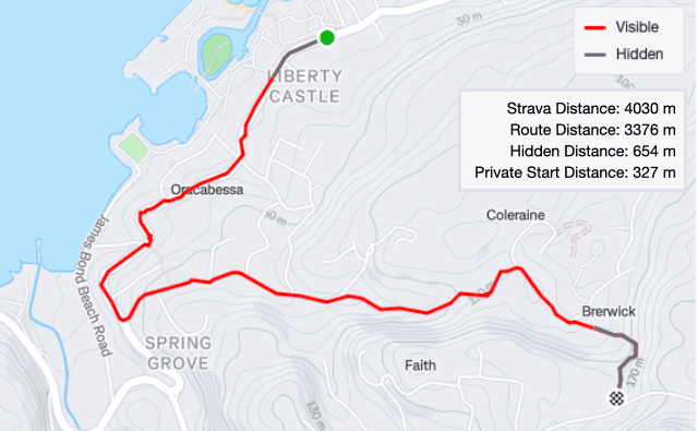
For reference: the blue cross marks the true start location and the white cross shows the predicted location using the homing method.
The homing method was almost spot on for this location: just 15m from the true start location. The privacy zone here might as well not exist. The geometric methods do reasonably well too, but mainly because the layout is simple - two clean clusters of start points on either side of the true start. Notice how the homing method is the only one that actually ends up on the road, that's because it's the only method that uses the road network itself to guide the prediction.
The next rural test showed a similar pattern, but with a larger gap. The best geometric methods landed 92.7m away; the homing method cut that in half, down to just 45m. Still not perfect, but a huge improvement - and in this environment, 45m is only a few buildings away.
The final location was the weakest of the bunch. The homing method was still the best, but only by a narrow margin: 79.7m from the true start, barely 6.7m better than the next best geometric method. Interestingly, the prediction is clearly being pulled in one direction, thanks to a slightly lopsided spread of start points.
Across all three additional rural locations, the pattern was the same: the homing method is always the best approach - often frighteningly good and much better than the geometric methods - but the accuracy varies depending on how the start points are distributed around the true start location.
And that distribution is not random. In each case where the method struggled, the start points were noticeably more spread out on one side than the other. That's the first sign something deeper is going on with how Strava applies its privacy zones. I'll dig into that next, because it turns out to matter quite a lot.
The Privacy-Zone Asymmetry Problem
We'd seen hints of this before, but the rural tests made it unmissable: whenever the homing method fell short, the start points weren't sitting at equal distances from the true start. One side would consistently be much closer, the other noticeably further away. And the more lopsided this was, the more it pulled the homing prediction off-centre.
This wasn't noise - it reflected how Strava applies its privacy zones.
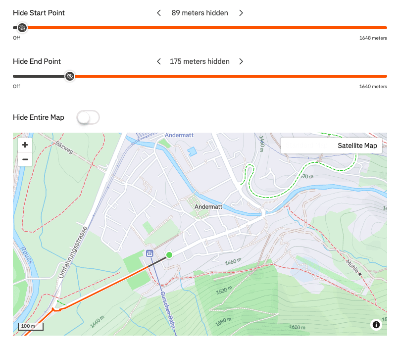
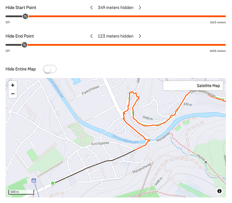
Inconsistent privacy zone sizes for the same start location in different directions
Strava doesn't hide the same distance at the start and end of an activity. In fact, the imbalance can be huge. Look at the example above for the rural 3 site, the left image shows an activity heading west had just 89m hidden at the start and 175m hidden at the end, a significant imbalance. Moreover, this isn't equal, the right image shows an activity starting at the same location but heading east, has 349m hidden at the start and 123m hidden at the end.
This is deliberate on Strava's part. If the hidden distance were always the same, reversing the privacy zone would be far too easy - you could simply measure the private distance and infer the radius. By varying the start and end lengths, they make the problem much harder. And it does help: the asymmetry is one of the few things that actually slows down the homing method.
But it's also predictable. That imbalance shows up directly in the start point clusters. The points closer to the true start location, where Strava hid a shorter distance, form tighter, more compact clusters. The startpoints where Strava hid more distance are more spread out. This is likely because more distance means more time for random errors to propagate, thus more difference in each start point.
So the key idea is simple:
- Tighter clusters should represent start points that were closer to the true start location.
- Looser clusters should represent start points that were further away.
Instead of blindly halving the hidden distance for every activity, we can weight the adjustment depending on how tight or loose each cluster is.
To do this, I used DBSCAN to group the start points into natural clusters (50m maximum spacing, minimum size of 3). For each cluster, I computed its standard deviation. Then I compared each cluster's spread to the average spread across all clusters to produce a "balancing factor":
- Tight clusters → factor less than 0.5
- Loose clusters → factor greater than 0.5
In short, tighter clusters pull the prediction towards the true start and looser clusters push it away, correcting the asymmetry that Strava builds into its privacy zones.
The balancing factor is computed as:
Using the example shown above, the western cluster ends up with a balancing factor of 0.43, and the eastern cluster 0.72. That means:
- The western cluster gets less than half its private distance (pulled closer to the true start).
- While the eastern cluster gets more than half (pushed further away).
This aligns far better with reality. Without any balancing, the estimated private distances for this example would be roughly 132m (west) and 236m (east). With balancing applied, they become 114m (west) and 340m (east) - much closer to Strava's actual behaviour of 89m and 349m.
This small tweak - just re-weighting the distances before running the homing method - turns out to make a remarkable difference. I'll show the results next.
Results With Balancing - A Huge Difference
With the balancing applied, the change in performance was immediate - and in some cases, ridiculously effective.
First, I reran the homing method with balancing on the original rural location. I wasn't expecting much improvement here; the homing method was already only 5.6m from the true start. But balancing surprised me and pulled it even closer - to under a metre, just 40cm away. I genuinely didn't think it could get any closer than it already was.
The second rural location showed the same trend. The original error was 15.0m, already impressive, yet balancing tightened this to 2.1m. That's staggeringly close - effectively at the front door. Balancing is clearly having a positive impact on the predictions.
The third rural example didn't improve in the same way. Here, the balancing nudged the prediction slightly further away (only by about 7m). This is because the furthest cluster from the true start was much more spread out than the others and ended up disproportionately influencing the correction. Human judgement could easily override this - it's visually obvious which cluster is the outlier - but algorithmically it's trickier. Still, this was a very small regression, not a failure.
The fourth rural location was the real test. Before balancing, the homing method was the best method, but only just - at ~80m from the true start. This location had the strongest start/end asymmetry of any example. After balancing, the prediction collapsed to 26m. That's a huge improvement and crucially, well within the distance of the true start that could be considered close. Bare in mind the next closest prediction was 86.4m!
This small adjustment - just rebalancing the distances before running the homing method - makes the results far scarier. In several cases the predicted start point closed in to within a few metres of the true start location and in one example it was under a metre away. Most of the others landed under 20m away and only a single test saw a slight worsening. Overall, once the start-end imbalance is corrected, the method becomes not only more consistent, but terrifyingly accurate.
Future Improvements
There are a few obvious directions to explore for improving the homing method. One is experimenting with different error metrics. While RMSE worked well in my tests, other metrics might provide more robust predictions in certain environments, especially where there are outliers or irregular start distributions.
Another area is exploring more advanced grid search strategies for the homing method. The current approach is simple and intuitive, but more sophisticated search methods could reduce computation time or improve accuracy in complex urban layouts. Further refinement of the balancing method for the homing method could also be explored - I think this can be improved further.
Machine learning could also play a role. For instance, a model could be trained to predict the hidden distance from the Strava metadata and map features. This could help address distortions caused by Strava's processing, particularly with larger privacy zones. More ambitiously, a model could learn patterns in Strava privacy zones themselves and incorporate these into the predictions. That said, the current method has already proven highly effective across the tests I've run and the challenges for getting a large dataset are likely insurmountable.
Finally, incorporating temporal metadata, like activity start times and speeds, could also provide additional context. At present I've only using distance, but elevation data could be informative too: if there's a difference in start and end elevation between possible routes, this could help pinpoint the true start by aligning with the terrain contours.
Wrapping Up - What This Means (And What's Next)
The homing method shows just how precise reverse-engineering can be. In rural and low-density areas, start locations can be pinpointed to within a few metres - essentially right up to someone's front door - while in cities the method still outperforms geometric approaches. And with balancing on the homing method, the accuracy becomes even more alarming, often narrowing the estimate to a handful of metres and in one case to within a single metre.
Larger privacy zones offer only the illusion of protection - even a handful of activities can reveal the true start location. It's frightening to realise that with just a few activities, a home can be located almost as accurately as if you were standing outside it.
With this knowledge in mind hopefully there's more understanding of the vulnerabilities in privacy zones. Be careful out there, at some point in the future I'll write-up some practical steps you can take to better protect yourself on Strava and similar platforms.